Data Science, Machine Learning and Statistical Models - MCGLM, a unified model for statistical analysis.

The Multivariate Covariance Generalized Linear Model (MCGLM) is a universalization of the classic statistical model GLM, widening for multivariate and non-independent response fitting. Due to its pliancy and explicit specification, this unified model can support many statistical analyses on a wide variety of data and distinct traits. Aiming to foment the pervasiveness of statistical analysis with MCGLM support, this essay instills MCGLM and its comprehensive new Python library - the mcglm. The library is hosted on PyPI and can be installed with the aid of some Python library manager, such as pip. https://pypi.org/project/mcglm/.

Introduction

Dated at the beginning of the 19th century and controversial about actual authorship, the least squares method established an optimization proposal [1]. According to the Gauss-Markov theorem [2], the resulting estimates are optimal and unbiased under linear conditions of continuous values. This optimization method is leveraged by linear regression, one of the primordial statistical models [3], [4]. A linear regression associates a response variable to a group of covariates by employing a linear operation on regression parameters [5]. Three main assumptions for linear regression are linearity, independent realizations of the response variable, and a gaussian homoscedastic error with a zero mean. Aiming to generalize it, some subsequential statistical proposals expanded these assumptions.

The Generalized Linear Model (GLM) [6] generalizes the gaussian assumption of linear regression to some models of the exponential family [7]; The Generalized Additive Model (GAM) [8] manages regression by the sum of smooth operations on covariates; The Generalized Estimating Equations (GEE) [9] applies the quasi-likelihood estimating functions to adjust longitudinal data; Copulas [10], [11] and Mixed Models [12] are consolidated models that can fit non-independent response data, to cite a few. Amid the most recent postulations resides the family of Multivariate Covariance Generalized Linear Models (MCGLM).

The Multivariate Covariance Generalized Linear Model (MCGLM) [13] universalizes GLM by allowing the multivariate analysis of non-independent responses, such as longitudinal and spatial data. This versatility is the main trait of MCGLM; it stems from two-moment assumptions and the specification of its five fundamental components: linear predictor via design matrix, link function, variance function, covariance link function, and the linear matrix predictor through Z matrices. The model allows the assessment of regression coefficients and dispersion parameters, hypothesis tests, goodness-of-fit measurements, and correlation coefficients between outcome variables.

Statistical models and a brief literary review.

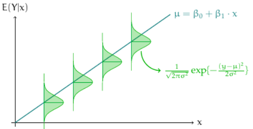
To develop intuition on statistical models, we dissect classical linear regression. According to McCullagh, P and Nelder, J.A, 1989 in their fantastic book “Generalized Linear Models”, yet rephrased by myself, an enthusiast disciple, a linear regression can be decomposed into two components: systematic and random parts.

Assuming an outcome variable $\boldsymbol{y}$ with $n$ components considered independent realizations of a random variable $\boldsymbol{Y}$. There is a vector $\boldsymbol{\mu}$ which holds the mean parameters of those realizations. The systematic part of the model specifies the vector $\boldsymbol{\mu}$ by employing a linear operation between regression parameters $\beta_0,...,\beta_p$ and the covariates. The mathematical notation for the systematic part:

\[\begin{equation*} \mathrm{E}(Y_i) = \mathrm{\mu_i} = \beta_0 + \sum_{j=1}^{p} x_{ij}\beta_j;\qquad i = 1,...,n. %\mathrm{V}(\boldsymbol{\mu}_r;p_r)^{\frac{1}{2}} (\boldsymbol{\Omega}(\boldsymbol{\tau}_r)) %\mathrm{V}(\boldsymbol{\mu}_r;p_r)^{\frac{1}{2}}. \end{equation*}\]

where $x_{ij}$ is the value of the jth covariate for observation $i$.

Moreover, as the random part, we assume independence and constant variance of errors. These errors follow a Gaussian distribution with mean 0 and constant variance $\sigma^2$ - giving to linear regression the adjective Homoscedasticity.

For a simple linear regression, the model graphically shapes as the image below:

As a statistical model, linear regression associates a response variable with at least one explanatory variable.

In 1972, Nelder and Wedderburn went a step further in unifying the theory of statistical modeling and, in particular, regression models, publishing their article on generalized linear models (GLM).

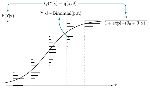
In the context of GLM, each component of the random variable $Y$ assumes a distribution in the exponential family, in which the probability or density function takes the form.

\[\begin{equation*} \mathrm{f}_y(y;\theta,\phi) = \mathrm{exp\{(y\theta - b(\theta))/a(\phi) + c(y,\phi)\}} \end{equation*}\]

for some specific functions $a(\phi)$, $b(\theta)$ and $c(y,\phi)$. Mean and Variance can be specified as:

\[\begin{equation*} \mathrm{E}(Y) = b'(\theta).\qquad \mathrm{Var}(Y) = b''(\theta)a(\phi). \end{equation*}\]

A couple of possible models in this framework:

\[\begin{array}{lll} \hline \text{Distribution} & \text{Support} & \text{Cases} \\ \hline \text{Gaussian} & \text{Real Numbers} & \text{General Symmetric Distributions.} \\ \text{Binomial(Bernoulli)} & \text{Bounded Data} & \text{Probability/Odds of an event.} \\ \text{Poisson} & \text{Integer Positive} & \text{Positive Count Distributions.} \\ \text{Gamma} & \text{Real Positive Numbers} & \text{Positive Asymmetric Distributions.} \\ \text{Inverse Gaussian} & \text{Real Positive Numbers} & \text{Positive Asymmetric Distributions.} \\ \hline \end{array}\]

GLM relies on three components: A design matrix with covariates, a link function, some distribution of exponential family or a variance function. The usual choices for the link and variance functions.

\[\begin{array}{lll} \hline \text{Distribution} & \text{Canonical link function} & \text{Variance function} \\ \hline \text{Poisson} & \text{Log} & \text{$\mu$} \\ \text{Binomial} & \text{Logit} & \text{$\mu(\mu - 1)$} \\ \text{Normal} & \text{Identity} & \text{1} \\ \text{Gamma} & \text{Reciprocal} & \text{$\mu^2$} \\ \text{Inverse Gaussian} & \text{Reciprocal²} & \text{$\mu^3$} \\ \hline \end{array}\]

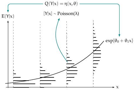
The maximum-likelihood estimator leverages the underlying distribution to find regression coefficients and dispersion estimates that maximize the product of likelihood. Therefore, two assumptions of GLM are: linearity upon the link function and random variable $Y$ is independently distributed as some exponential family distribution. The figure below illustrates the Binomial and Poisson models.

Stepping ahead two years, Wedderburn, one of the authors of GLM, published in 1974 one of the most iconic papers of history. “Quasi-Likelihood Functions, Generalized Linear Models, and the Gauss-Newton Method”. He proposed a relative likelihood estimator, the quasi-likelihood, which does not rely on a distribution model, yet provides asymptotically unbiased and consistent estimators. As long as statisticians cannot know the distribution upfront, the quasi-likelihood play an essential role in statistical models. The quasi-score is an Estimating Equation for quasi-likelihood functions.

In 1986, Liang and Zeger published the paper “Longitudinal data analysis using generalized linear models”, which establishes an extension of Generalized Linear Models (GLM) to longitudinal data analysis. The paper epitomizes that data scenario.

The severity of respiratory disease, along with the nutritional status, age, and family income of children, might be observed once every three months for 18 months. The dependence of the outcome variable, severity of disease, on the covariates is of interest.

The paper introduces an Estimating Equation that gives consistent estimates of the regression coefficients and their variances under weak assumptions about the joint distribution, the model GEE. The dispersion parameters remain a nuisance. The model harnesses the correlation matrix to define the dependence between components of the response variable. Furthermore, the paper suggests some dependences structures for GEE: independent, autoregressive, exchangeable, unstructured, stationary-M, M-dependent, or non-stationary. The GEE relies on the specification of four components: design matrix with covariates; link function; variance function; correlation matrix.

Finally, in 2016, Bonat and Jørgensen published the MCGLM, A brand new family of Statistical Models: Multivariate Covariance Generalized Linear Models.

MCGLM

The two-moment assumptions entail distinct apparatus for mean and variance. The optimization process of MCGLM blends two second-order optimization algorithms, the Fisher Scoring [14], [15] for regression, and Chaser [16] for dispersion parameters in tandem. Moreover, the estimating functions Quasi-score [17] and Pearson Estimating Equation are leveraged for the first and second moment, respectively.

Let $\mathbf{Y}_{N \times R} = \{\boldsymbol{Y}_1, \ldots, \boldsymbol{Y}_R\}$ be a response matrix, and $\mathbf{M}_{N \times R} = \{\boldsymbol{\mu}_1, \ldots, \boldsymbol{\mu}_R\}$ denote the corresponding matrix of expected values. Let $\boldsymbol{\Sigma}_r$ the $N \times N$ variance-covariance matrix of the outcome $r$, for $r = 1, \ldots, R$. Similarly, let $\boldsymbol{\Sigma}_b$ be a $R \times R$ correlation matrix inter responses. Let $\boldsymbol{X}_r$ denote an $N k_r $ design matrix and $\boldsymbol{\beta}_r$ a $k_r \times 1$ regression parameter vector. The two-moment specification of the MCGLM model goes as it follows:

\[\begin{equation*} \mathrm{E}(\mathbf{Y}) = \mathbf{M} = \{g_1^{-1}(\boldsymbol{X}_1 \boldsymbol{\beta}_1), \ldots, g_R^{-1}(\boldsymbol{X}_R \boldsymbol{\beta}_R)\} \end{equation*}\]

\[\begin{equation*} \mathrm{Var}(\mathbf{Y}) = \boldsymbol{C} = \boldsymbol{\Sigma}_R \overset{G} \otimes \boldsymbol{\Sigma}_b \end{equation*}\]

where the $C$ leverages the generalized Kronecker product $\boldsymbol{\Sigma}_R \overset{G} \otimes \boldsymbol{\Sigma}_b = \mathrm{Bdiag}(\tilde{\boldsymbol{\Sigma}}_1, \ldots, \tilde{\boldsymbol{\Sigma}}_R)(\boldsymbol{\Sigma}_b \otimes \boldsymbol{I})\mathrm{Bdiag}(\tilde{\boldsymbol{\Sigma}}_1^T, \ldots, \tilde{\boldsymbol{\Sigma}}_R^T)$ [18]. The matrix $\tilde{\boldsymbol{\Sigma}}_r$ denotes a low triangular Cholesky decomposition of $\boldsymbol{\Sigma}_r$. The operator $\mathrm{Bdiag}$ denotes a block diagonal matrix and $\boldsymbol{I}$ denotes an $N \times N$ identity matrix. Regarding the mean, or expectation, operation $g_r(\cdot)$ is a usual link function from GLM. $\boldsymbol{\Sigma}_r$ is defined by:

\[\begin{equation*} \boldsymbol{\Sigma}_r = \mathrm{V}(\boldsymbol{\mu}_r;p_r)^{\frac{1}{2}} (\boldsymbol{\Omega}(\boldsymbol{\tau}_r)) \mathrm{V}(\boldsymbol{\mu}_r;p_r)^{\frac{1}{2}}, \end{equation*}\] where $\mathrm{V}(\boldsymbol{\mu}_r;p_r) = \mathrm{diag}(\vartheta(\boldsymbol{\mu}_r;p_r))$ is a diagonal matrix, whose main entries are the variance function applied on the expected values $\boldsymbol{\mu_r}$. Each variance function establishes its unique marginal distributions on MCGLM. Furthermore, MCGLM leverages linear matrix predictor with covariance link function for dispersion matrix definition [19], [20], [21]. \[\begin{equation} h(\boldsymbol{\Omega}(\boldsymbol{\tau}_r)) = \tau_{r0} Z_{r0} + \cdots + \tau_{rD} Z_{rD}, \end{equation}\]

where $\mathrm{h(\cdot)}$ is the covariance link function and matrices $Z_r$ specifies the dependence inner response. The main article details many structures that can be fitted through linear matrix predictor.

As the mathematical notation alludes, it is up to the user to pick their choices for the link, variance, covariance functions, and dependence matrices.

MCGLM components

The variance function is fundamental to the MCGLM, as it defines the marginal distribution of a response variable. To highlight some common choices, the variance function power specializes in handling continuous data and is fundamental to the Tweedie family of distribution models. According to [23] and [24], this family has its emblematic cases: Gaussian (p = 0), Gamma (p = 2), and Inverse Gaussian (p = 3). The variance function extended binomial is a common choice for analyzing limited data. For the adjustment of count data, the dispersion function presented by [25], called Poisson-Tweedie, is flexible to capture notable models, such as: Hermite (p = 0), Neyman Type A (p = 1), Negative Binomial (p = 2) and Gaussian Poisson-inverse (p = 3). The following table summarizes the variance functions cited:

\[\begin{array}{ll} \hline \text{Function name} & \text{Formula} \\ \hline \text{power/Tweedie} & \mathrm{V}(p) = \mu^{p} \\ \text{binomial} & \mathrm{V}(p) = \mu^{p} (1 - \mu_r)^{p} \\ \text{Poisson-Tweedie} & \mathrm{V}(p) = \mu + \tau\mu_{p} \\ \hline \end{array}\]

The covariance link function $h(\cdot)$ is described by . To cite a few examples: identity, inverse and exponential-matrix [22].

In MCGLM, the user specifies the dependency through dependency matrices Z, supporting the flexible profile of the model. Many classical statistical models are replicable by specifying Z matrices. To cite a few, mixed models, moving averages and compound symmetry. For in-deep details, see [13].

The brand new library mcglm.

The Python library mcglm provides an easy interface for fitting the MCGLM model, similar to the library statsmodels, providing auxiliary methods to lead a proper specification of each MCGLM component. The library provides a comprehensive report for the model fitting analysis with regression coefficients, dispersion estimates, confidence intervals, hypothesis testing, and Pearson residuals. Only R users have access to the MCGLM algorithm by the package mcglm.

Finally, this notebook presents some statistical analysis with the support of Python mcglm.

Refs:

https://www.jstor.org/stable/44681850
https://www.researchgate.net/publication/324579147_Multiple_Response_Variables_Regression_Models_in_R_The_mcglm_Package

Modeling time

Code

import sys
import os

import statsmodels.api as sm
import pandas as pd
import matplotlib.pyplot as plt
import seaborn as sns
import numpy as np

sys.path.append(os.path.join(sys.path[0], ".."))

from mcglm import MCGLM, mc_mixed, mc_id, mc_ma
from patsy import dmatrix
from statsmodels.tools.tools import add_constant
from statsmodels.tsa.seasonal import seasonal_decompose
from statsmodels.tsa.stattools import adfuller
from statsmodels.tsa.arima_process import ArmaProcess

import warnings

warnings.simplefilter("ignore")

Code

# library docstring.
print(MCGLM.__doc__)


    MCGLM class that implements MCGLM stastical models. (Bonat, Jørgensen 2015)
        
    It extends GLM for multi-responses and dependent components by fitting second-moment assumptions.

    Parameters
    ----------
    endog : array_like
        1d array of endogenous response variable. In case of multiple responses, the user must pass the responses on a list.  
    exog : array_like
        A dataset with the endogenous matrix in a Numpy fashion. Since the library doesn't set an intercept by default, the user must add it. In the case of multiple responses, the user must pass the design matrices as a python list. 
    z : array_like
        List with matrices components of the linear covariance matrix.
    link : array_like, string or None
        Specification for the link function. The MCGLM library implements the following options: identity, logit, power, log, probit, cauchy, cloglog, loglog, negativebinomial. In the case of None, the library chooses the identity link. In multiple responses, user must pass values as list.  
    variance : array_like, string or None
        Specification for the variance function. The MCGLM library implements the following options: constant, tweedie, binomialP, binomialPQ, geom_tweedie, poisson_tweedie. In the case of None, the library chooses the constant link. In multiple responses, user must pass values as list.   
    offset : array_like or None
        Offset for continuous or count. In multiple responses, user must pass values as list.   
    Ntrial : array_like or None
        Ntrial for binomial responses. In multiple responses, user must pass values as list.
    power_fixed : array_like or None
        Parameter that allows estimation of power when variance functions is either tweedie, geom_tweedie or poisson_tweedie. In multiple responses, user must pass values as list. 
    maxiter : float or None
        Number max of iterations. Defaults to 200.
    tol : float or None
        Threshold of minimum absolute change on paramaters. Defaults to 0.0001.
    tuning : float or None
        Step size parameter. Defaults to 0.5.
    weights : array_like or None
        Weight matrix. Defaults to None.
        
    Examples
    ----------
    >>> import statsmodels.api as sm
    >>> data = sm.datasets.scotland.load()
    >>> data.exog = sm.add_constant(data.exog)
    
    >>> model = sm.GLM(data.endog, data.exog, z=[mc_id(data.exog)],
    ...                      link="log", variance="tweedie",
    ...                      power=2, power_fixed=False)
    
    >>> model_results = model.fit()
    >>> model_results.mu
    >>> model_results.pearson_residuals
    >>> model_results.aic
    >>> model_results.bic
    >>> model_results.loglikelihood
    
    Notes
    -----
    MCGLM is a brand new model, which provides a solid statistical model for fitting multi-responses non-gaussian, dependent, or independent data based on second-moment assumptions. When a user instantiates an mcglm object, she must specify attributes such as link, variance, and z matrices; it will drive the overall behavior of the model.
    For more details, check articles and documentation provided.

To instill mcglm, we begin with statistical analysis of i.i.d(independent and identically distributed) outcomes. For that, components Z will be specified as identity matrices, using method mc_id(). Upcoming examples epitomize the flexibility of mcglm in fitting different distribution models.

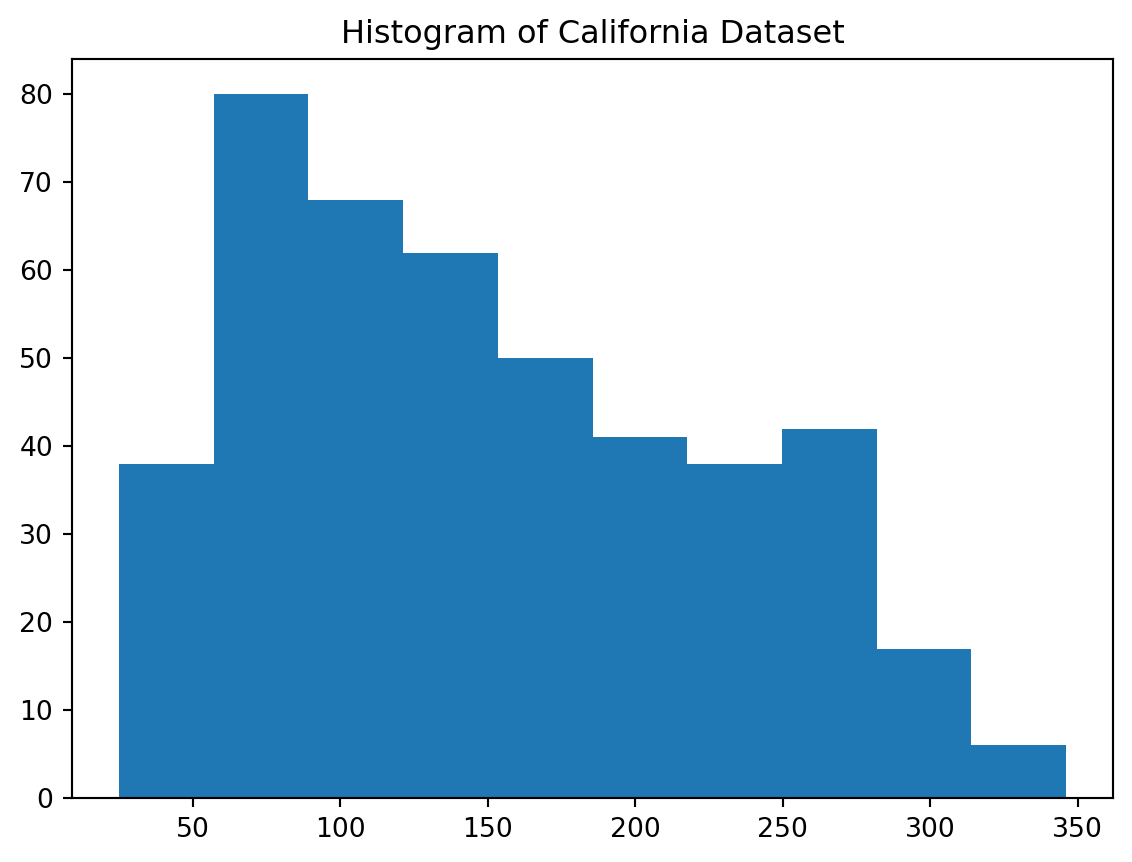
1. Diabetes dataset

Diabetes dataset outputs suited for regression modeling.

Code

from sklearn.datasets import load_diabetes

X, y = load_diabetes(return_X_y=True)
X = pd.DataFrame(X)
y = pd.Series(y, name="output")


# looking at target distribution
_ = plt.hist(y)
plt.title("Histogram of California Dataset")

Text(0.5, 1.0, 'Histogram of California Dataset')

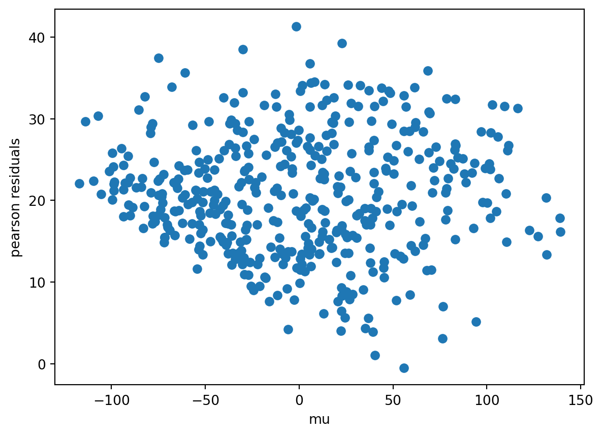
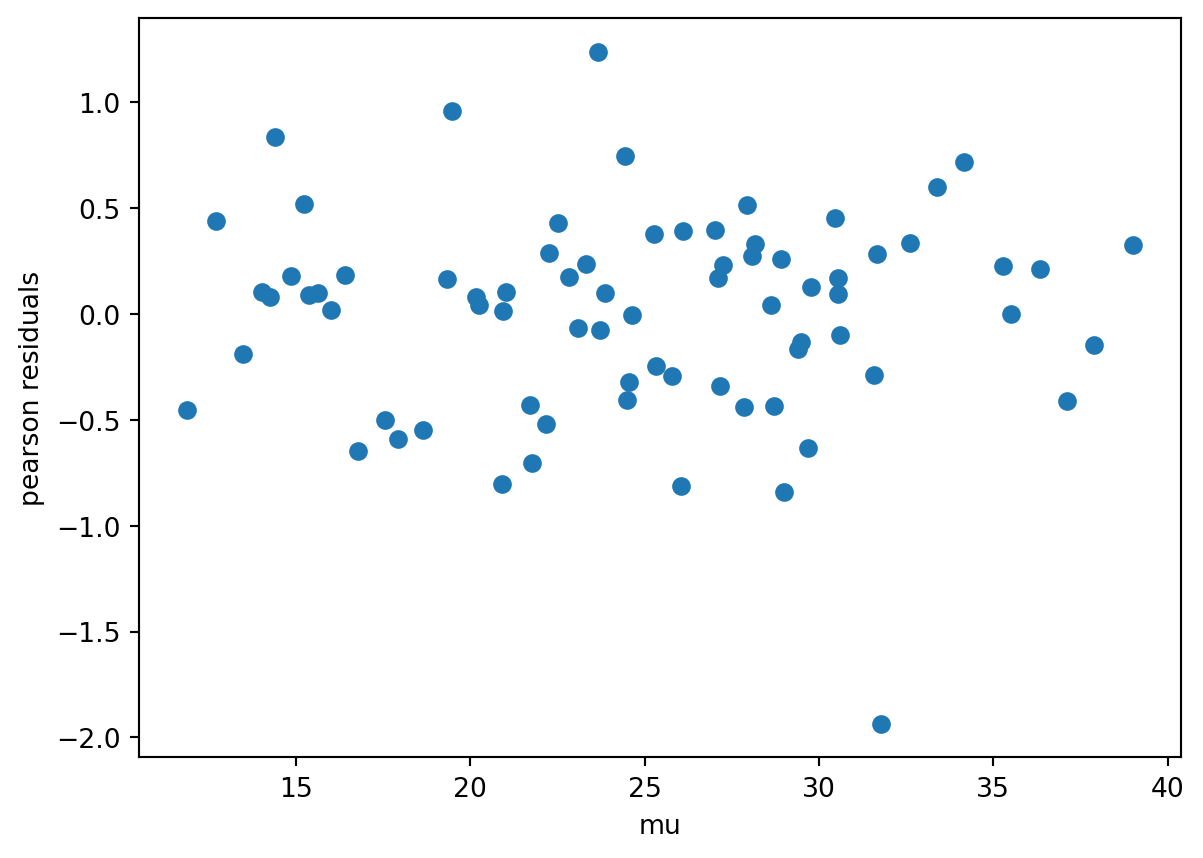
Starting with linear regression, fitting a linear regression through the mcglm library is plain. The picks are identity as a link, constant as variance, and an identity matrix as Z.

Code

modelresults = MCGLM(endog=y, 
                     exog=X, 
                     z=[mc_id(X)]
                     ).fit()

[modelresults.summary()]

[<class 'statsmodels.iolib.summary.Summary'>
 """
                Multivariate Covariance Generalized Linear Model               
 ==============================================================================
 Dep. Variable:                 output   No. Iterations:                      1
 Model:                          MCGLM   No. Observations:                  442
 link:                        identity   Df Residuals:                      431
 variance:                    constant   Df Model:                           11
 Method:              Quasi-Likelihood   Power-fixed:                      True
 Date:                Mon, 06 Feb 2023   pAIC                           5327.73
 Time:                        07:45:45   pBIC                           5372.73
                                         pLogLik                     -2652.8628
 ==============================================================================
                  coef    std err          z      P>|z|      [0.025      0.975]
 ------------------------------------------------------------------------------
 0            -10.0099    177.919     -0.056      0.955    -358.725     338.705
 1           -239.8156    182.306     -1.315      0.188    -597.128     117.497
 2            519.8459    198.121      2.624      0.009     131.536     908.156
 3            324.3846    194.811      1.665      0.096     -57.438     706.208
 4           -792.1756   1240.774     -0.638      0.523   -3224.047    1639.696
 5            476.7390   1009.552      0.472      0.637   -1501.947    2455.425
 6            101.0433    632.868      0.160      0.873   -1139.356    1341.442
 7            177.0632    480.837      0.368      0.713    -765.359    1119.486
 8            751.2737    511.877      1.468      0.142    -251.987    1754.535
 9             67.6267    196.486      0.344      0.731    -317.478     452.731
 ================================================================================
                    coef    std err          z      P>|z|      [0.025      0.975]
 --------------------------------------------------------------------------------
 dispersion_1    2.6e+04    796.484     32.649      0.000    2.44e+04    2.76e+04
 ==============================================================================
                  coef    std err          z      P>|z|      [0.025      0.975]
 ------------------------------------------------------------------------------
 power_         1.0000        nan        nan        nan         nan         nan
 ==============================================================================
 """]

The residual analysis is key for assessing the fulfillment of the assumptions. For more details, check out (Montgomery. D.C and Runger. G.C, 2013).

Code

# Residual Analysis
plt.scatter(modelresults.mu, modelresults.pearson_residuals)
plt.xlabel("mu")
plt.ylabel("pearson residuals")

Text(0, 0.5, 'pearson residuals')

As long as the Pearson residuals aren’t shapeless, they may point to a non-optimal fitting.

2. A count analysis

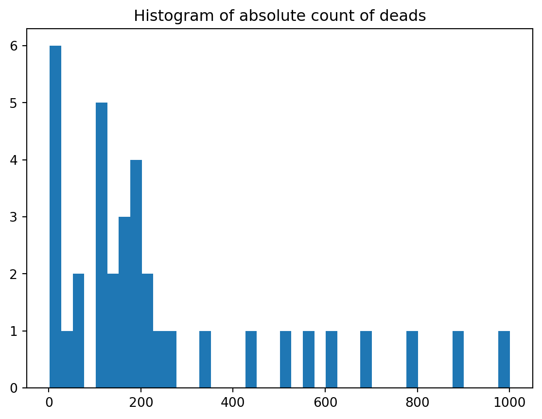
This dataset hosts information from a Canadian study of mortality by age and smoking status. https://data.princeton.edu/wws509/datasets/#smoking. The four-column dataset establishes features: age, smoking status, population, and the outcome of deaths.

Linear regression is unsuitable for analyzing discrete count data, and a Poisson model is a usual choice. With mcglm is easy to leverage the Poisson Model.

Code

smoking_data = pd.read_csv("data/smoking_data.csv")

## exog and endog
X = dmatrix("~ pop + age + smoke", smoking_data, return_type="dataframe")
y = smoking_data["dead"]

Code

_ = plt.hist(y, bins=40)
plt.title("Histogram of absolute count of deads")

Text(0.5, 1.0, 'Histogram of absolute count of deads')

That is a long-tail distribution.

Straight off the bat, we attempt fitting as a linear regression: identity and constant.

Code

modelresults = MCGLM(
    y,
    X,
    [mc_id(X)],
).fit()

[modelresults.summary()]

[<class 'statsmodels.iolib.summary.Summary'>
 """
                Multivariate Covariance Generalized Linear Model               
 ==============================================================================
 Dep. Variable:                   dead   No. Iterations:                      1
 Model:                          MCGLM   No. Observations:                   36
 link:                        identity   Df Residuals:                       22
 variance:                    constant   Df Model:                           14
 Method:              Quasi-Likelihood   Power-fixed:                      True
 Date:                Mon, 06 Feb 2023   pAIC                            429.44
 Time:                        07:45:46   pBIC                            451.61
                                         pLogLik                       -200.719
 =============================================================================================
                                 coef    std err          z      P>|z|      [0.025      0.975]
 ---------------------------------------------------------------------------------------------
 Intercept                  -224.6373     66.931     -3.356      0.001    -355.820     -93.455
 age[T.45-59]                 95.3834     76.446      1.248      0.212     -54.448     245.215
 age[T.50-54]                147.8634     78.491      1.884      0.060      -5.977     301.703
 age[T.55-59]                216.4651     74.395      2.910      0.004      70.654     362.276
 age[T.60-64]                344.0038     76.451      4.500      0.000     194.162     493.846
 age[T.65-69]                426.7793     74.466      5.731      0.000     280.829     572.730
 age[T.70-74]                399.1722     78.027      5.116      0.000     246.242     552.103
 age[T.75-79]                335.9303     83.318      4.032      0.000     172.629     499.231
 age[T.80+]                  293.7420     86.312      3.403      0.001     124.573     462.911
 smoke[T.2.cigarPipeOnly]     32.3389     49.616      0.652      0.515     -64.906     129.584
 smoke[T.3.cigarrettePlus]    85.2001     76.811      1.109      0.267     -65.347     235.747
 smoke[T.4.cigarretteOnly]    87.8965     60.879      1.444      0.149     -31.425     207.218
 pop                           0.1128      0.023      4.814      0.000       0.067       0.159
 ================================================================================
                    coef    std err          z      P>|z|      [0.025      0.975]
 --------------------------------------------------------------------------------
 dispersion_1  1.107e+04   1899.730      5.825      0.000    7342.638    1.48e+04
 ==============================================================================
                  coef    std err          z      P>|z|      [0.025      0.975]
 ------------------------------------------------------------------------------
 power_         1.0000        nan        nan        nan         nan         nan
 ==============================================================================
 """]

Let’s try a Tweedie with a power set as one, as a Poisson model. As mentioned, Poisson is a suitable pick for modeling count data.

Code

modelresults = MCGLM(
    y,
    X,
    [mc_id(X)],
    link="log",
    variance="tweedie",
    power=1,
    power_fixed=True,
).fit()

[modelresults.summary()]

[<class 'statsmodels.iolib.summary.Summary'>
 """
                Multivariate Covariance Generalized Linear Model               
 ==============================================================================
 Dep. Variable:                   dead   No. Iterations:                      1
 Model:                          MCGLM   No. Observations:                   36
 link:                             log   Df Residuals:                       22
 variance:                     tweedie   Df Model:                           14
 Method:              Quasi-Likelihood   Power-fixed:                      True
 Date:                Mon, 06 Feb 2023   pAIC                            371.22
 Time:                        07:45:46   pBIC                            393.39
                                         pLogLik                      -171.6087
 =============================================================================================
                                 coef    std err          z      P>|z|      [0.025      0.975]
 ---------------------------------------------------------------------------------------------
 Intercept                     2.5604      0.283      9.056      0.000       2.006       3.115
 age[T.45-59]                  0.6242      0.310      2.011      0.044       0.016       1.233
 age[T.50-54]                  1.0038      0.308      3.261      0.001       0.401       1.607
 age[T.55-59]                  1.3818      0.245      5.635      0.000       0.901       1.862
 age[T.60-64]                  1.5012      0.245      6.133      0.000       1.021       1.981
 age[T.65-69]                  2.1366      0.240      8.920      0.000       1.667       2.606
 age[T.70-74]                  2.3557      0.269      8.766      0.000       1.829       2.882
 age[T.75-79]                  2.2041      0.298      7.403      0.000       1.621       2.788
 age[T.80+]                    1.9506      0.318      6.143      0.000       1.328       2.573
 smoke[T.2.cigarPipeOnly]      0.2114      0.176      1.203      0.229      -0.133       0.556
 smoke[T.3.cigarrettePlus]     0.5030      0.214      2.347      0.019       0.083       0.923
 smoke[T.4.cigarretteOnly]     0.7818      0.164      4.755      0.000       0.460       1.104
 pop                           0.0004   6.25e-05      6.679      0.000       0.000       0.001
 ================================================================================
                    coef    std err          z      P>|z|      [0.025      0.975]
 --------------------------------------------------------------------------------
 dispersion_1    14.1200      3.786      3.729      0.000       6.699      21.541
 ==============================================================================
                  coef    std err          z      P>|z|      [0.025      0.975]
 ------------------------------------------------------------------------------
 power_         1.0000        nan        nan        nan         nan         nan
 ==============================================================================
 """]

Code

# Residual Analysis
plt.scatter(modelresults.mu, modelresults.pearson_residuals)
plt.xlabel("mu")
plt.ylabel("pearson residuals")

Text(0, 0.5, 'pearson residuals')

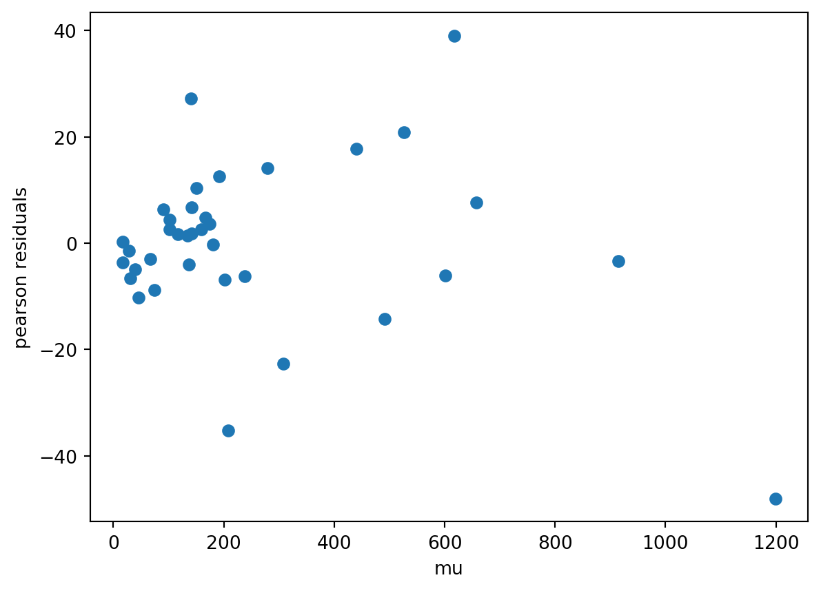
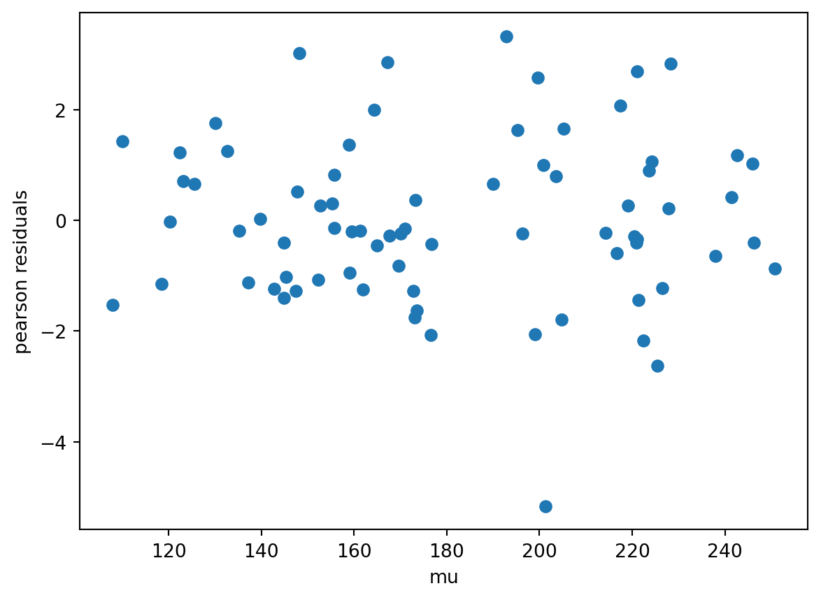
By the pAIC metric, the usual Tweedie variance function is a suitable pick.

It is plain to harness an essential trait of the mcglm library, the power estimation for a Poisson Tweedie fitting. We have got to set the parameter power_fixed as False.

Code

modelresults = MCGLM(
    y,
    X,
    [mc_id(X)],
    link="log",
    variance="poisson_tweedie",
    power=1,
    power_fixed=False,
).fit()

[modelresults.summary()]

[<class 'statsmodels.iolib.summary.Summary'>
 """
                Multivariate Covariance Generalized Linear Model               
 ==============================================================================
 Dep. Variable:                   dead   No. Iterations:                     12
 Model:                          MCGLM   No. Observations:                   36
 link:                             log   Df Residuals:                       22
 variance:             poisson_tweedie   Df Model:                           14
 Method:              Quasi-Likelihood   Power-fixed:                     False
 Date:                Mon, 06 Feb 2023   pAIC                            370.17
 Time:                        07:45:46   pBIC                            392.34
                                         pLogLik                      -171.0843
 =============================================================================================
                                 coef    std err          z      P>|z|      [0.025      0.975]
 ---------------------------------------------------------------------------------------------
 Intercept                     2.4466      0.269      9.094      0.000       1.919       2.974
 age[T.45-59]                  0.6573      0.297      2.209      0.027       0.074       1.240
 age[T.50-54]                  1.0419      0.298      3.498      0.000       0.458       1.626
 age[T.55-59]                  1.3900      0.244      5.703      0.000       0.912       1.868
 age[T.60-64]                  1.5253      0.242      6.300      0.000       1.051       2.000
 age[T.65-69]                  2.1935      0.236      9.283      0.000       1.730       2.657
 age[T.70-74]                  2.4571      0.263      9.350      0.000       1.942       2.972
 age[T.75-79]                  2.3416      0.290      8.082      0.000       1.774       2.909
 age[T.80+]                    2.1177      0.307      6.906      0.000       1.517       2.719
 smoke[T.2.cigarPipeOnly]      0.1685      0.172      0.980      0.327      -0.168       0.505
 smoke[T.3.cigarrettePlus]     0.4427      0.217      2.041      0.041       0.017       0.868
 smoke[T.4.cigarretteOnly]     0.7345      0.167      4.398      0.000       0.407       1.062
 pop                           0.0005    6.4e-05      7.110      0.000       0.000       0.001
 ================================================================================
                    coef    std err          z      P>|z|      [0.025      0.975]
 --------------------------------------------------------------------------------
 dispersion_1     3.0590      3.121      0.980      0.327      -3.059       9.177
 ==============================================================================
                  coef    std err          z      P>|z|      [0.025      0.975]
 ------------------------------------------------------------------------------
 power_         1.2895      0.198      6.526      0.000       0.902       1.677
 ==============================================================================
 """]

By the pAIC, the adjustment with Poisson Tweedie power set 1.263 is lightly better than Poisson 1. It points out that the distribution Poisson Tweedie is the best option for this data learning.

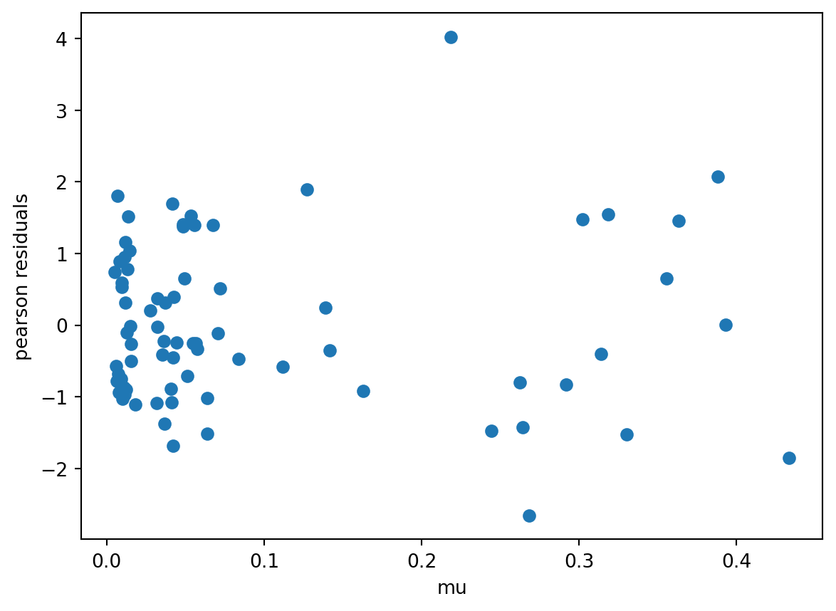
3. A bounded analysis

For a bound analysis, we analyze the iconic titanic dataset.

Code

titanic = pd.read_csv("data/titanic.csv")

y = titanic["Survived"]

X = titanic[["Fare", "SibSp", "Embarked", "Parch", "Pclass"]]
X = X.fillna("S")

X = dmatrix("~ Fare + SibSp + Embarked + Parch + Pclass", X, return_type="dataframe")

modelresults = MCGLM(
    y,
    X,
    [mc_id(X)],
    link="logit",
    variance="binomialP",
    ntrial=1,
).fit()
[modelresults.summary()]

[<class 'statsmodels.iolib.summary.Summary'>
 """
                Multivariate Covariance Generalized Linear Model               
 ==============================================================================
 Dep. Variable:               Survived   No. Iterations:                      1
 Model:                          MCGLM   No. Observations:                  891
 link:                           logit   Df Residuals:                      883
 variance:                   binomialP   Df Model:                            8
 Method:              Quasi-Likelihood   Power-fixed:                      True
 Date:                Mon, 06 Feb 2023   pAIC                            212.54
 Time:                        07:45:48   pBIC                            250.88
                                         pLogLik                       -98.2698
 =================================================================================
                     coef    std err          z      P>|z|      [0.025      0.975]
 ---------------------------------------------------------------------------------
 Intercept         1.4120      0.343      4.122      0.000       0.741       2.083
 Embarked[T.Q]     0.2911      0.307      0.949      0.343      -0.310       0.893
 Embarked[T.S]    -0.5179      0.196     -2.636      0.008      -0.903      -0.133
 Fare              0.0037      0.002      1.554      0.120      -0.001       0.008
 SibSp            -0.1274      0.082     -1.561      0.119      -0.287       0.033
 Parch             0.2920      0.101      2.906      0.004       0.095       0.489
 Pclass           -0.7556      0.116     -6.508      0.000      -0.983      -0.528
 ================================================================================
                    coef    std err          z      P>|z|      [0.025      0.975]
 --------------------------------------------------------------------------------
 dispersion_1     0.9990      0.036     27.961      0.000       0.929       1.069
 ==============================================================================
                  coef    std err          z      P>|z|      [0.025      0.975]
 ------------------------------------------------------------------------------
 power_         1.0000        nan        nan        nan         nan         nan
 ==============================================================================
 """]

Code

## Evaluating multiple links
modelresults_logit = MCGLM(
    y, X, [mc_id(X)], link="logit", variance="binomialP", ntrial=1
).fit()

modelresults_loglog = MCGLM(
    y, X, [mc_id(X)], link="loglog", variance="binomialP", ntrial=1
).fit()

modelresults_cloglog = MCGLM(
    y, X, [mc_id(X)], link="cloglog", variance="binomialP", ntrial=1
).fit()

modelresults_cauchy = MCGLM(
    y, X, [mc_id(X)], link="cauchy", variance="binomialP", ntrial=1
).fit()

Code

print(
    "logit_aic: ",
    modelresults_logit.aic,
    ", loglog_aic: ",
    modelresults_loglog.aic,
    ", cloglog_aic: ",
    modelresults_cloglog.aic,
    ", cauchy_aic: ",
    modelresults_cauchy.aic,
)

logit_aic:  212.54 , loglog_aic:  202.04 , cloglog_aic:  222.58 , cauchy_aic:  216.94

The loglog link is the best pick for this analysis.

In addition, the mcglm can fit response variables when its realizations are non-independent.

Non-independent section

Let’s leverage the mcglm to adjust non-independent data, illustrated by a Moving Average and Mixed Model analysis, two iconic statistical models.

1. Moving Average model

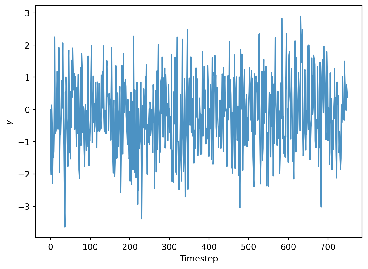
In MA model, the current realization is linearly dependent of past error terms. The script below defines a MA realization of size 1, and q defined as 0.4.

Code

SAMPLE_SIZE = 750
RANDOM_SEED = 42
y = np.zeros((SAMPLE_SIZE,))


# true stationarity
true_theta = 0.4
# true standard deviation of the innovation:
true_sigma = 1
# true process mean:
true_center = 0.0

innovations = np.random.normal(true_center, true_sigma, SAMPLE_SIZE)

for t in range(1, SAMPLE_SIZE):
    y[t] = innovations[t] + true_theta * innovations[t-1]

plt.plot(y, alpha=0.8)
plt.xlabel("Timestep")
plt.ylabel("$y$")

Text(0, 0.5, '$y$')

Code

# building covariance matrix and outcome vector.
data = pd.DataFrame()
data["ma_sample"] = y
data["index"] = list(range(0, SAMPLE_SIZE))
data = add_constant(data)

X = data[["const"]]
y = data["ma_sample"]

To find the best size for MA, the q fitting, we benchmark them by pAIC. Moreover, the mc_ma assist us in building the Z matrices for the MA analysis.

Code

one_order = [mc_id(X), mc_ma(id="const", time="index", data=data, order=1)]
two_order = [*one_order, mc_ma(id="const", time="index", data=data, order=2)]
three_order = [*two_order, mc_ma(id="const", time="index", data=data, order=3)]
four_order = [*three_order, mc_ma(id="const", time="index", data=data, order=4)]
five_order = [*four_order, mc_ma(id="const", time="index", data=data, order=5)]
six_order = [*five_order, mc_ma(id="const", time="index", data=data, order=6)]
seven_order = [*six_order, mc_ma(id="const", time="index", data=data, order=7)]

Code

for index, order in enumerate(
    [one_order, two_order, three_order, four_order, five_order, six_order, seven_order]
):
    modelresults = MCGLM(y, X, order).fit()

    print("q value: ", str(index + 1), ", paic: ", modelresults.aic)

q value:  1 , paic:  1422.59

q value:  2 , paic:  1422.62

q value:  3 , paic:  1423.01

q value:  4 , paic:  1425.0

q value:  5 , paic:  1426.85

q value:  6 , paic:  1428.11

q value:  7 , paic:  1428.6

Displacement q as 1 as the best fit.

Code

modelresults = MCGLM(y, X, one_order).fit()
[modelresults.summary()]

[<class 'statsmodels.iolib.summary.Summary'>
 """
                Multivariate Covariance Generalized Linear Model               
 ==============================================================================
 Dep. Variable:              ma_sample   No. Iterations:                      3
 Model:                          MCGLM   No. Observations:                  750
 link:                        identity   Df Residuals:                      747
 variance:                    constant   Df Model:                            3
 Method:              Quasi-Likelihood   Power-fixed:                      True
 Date:                Mon, 06 Feb 2023   pAIC                           1422.59
 Time:                        07:47:22   pBIC                           1436.45
                                         pLogLik                      -708.2965
 ==============================================================================
                  coef    std err          z      P>|z|      [0.025      0.975]
 ------------------------------------------------------------------------------
 const         -0.1389      0.053     -2.598      0.009      -0.244      -0.034
 ================================================================================
                    coef    std err          z      P>|z|      [0.025      0.975]
 --------------------------------------------------------------------------------
 dispersion_1     1.2450      0.066     18.987      0.000       1.116       1.374
 dispersion_2     0.4510      0.042     10.799      0.000       0.369       0.533
 ==============================================================================
                  coef    std err          z      P>|z|      [0.025      0.975]
 ------------------------------------------------------------------------------
 power_         1.0000        nan        nan        nan         nan         nan
 ==============================================================================
 """]

The summary report drills down the $\theta$ parameters that linearly operate the Gaussian White Noise, and 0.4, the actual value, falls within the interval of the second dispersion parameter.

2. Random Effect models

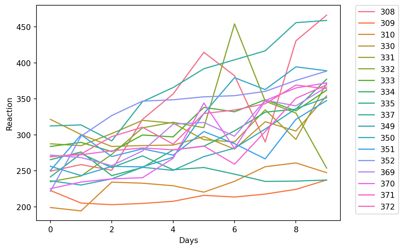
The dataset sleepstudy is a study of sleep deprivation. https://www.rdocumentation.org/packages/lme4/versions/1.1-26/topics/sleepstudy.

The study aims to understand the influence of sleep deprivation on reaction time. On day 0, subjects had their usual amount of sleep. From day 0 on, they were restricted to 3 hours of sleep per night. The observations represent the average reaction time on a series of tests given each day to each subject.

One promising approach is fitting through two-level effect models, such as mixed models. The mcglm library is a perfect framework to apply this statistical learning; due to the model and the method mc_mixed() to build a dependence matrix.

Code

# Top 10 cells to get an intuition about data.
sleepstudy = pd.read_csv(
    "data/first_simulation/sleepstudy.csv", dtype={"Subject": "str"}
)

sleepstudy.head(10)

	Reaction	Days	Subject
0	249.5600	0	308
1	258.7047	1	308
2	250.8006	2	308
3	321.4398	3	308
4	356.8519	4	308
5	414.6901	5	308
6	382.2038	6	308
7	290.1486	7	308
8	430.5853	8	308
9	466.3535	9	308

Code

## Plotting curve of 18 subjects
_ = sns.lineplot(x="Days", y="Reaction", hue="Subject", data=sleepstudy)
plt.legend(bbox_to_anchor=(1.05, 1), loc=2, borderaxespad=0.0)

<matplotlib.legend.Legend at 0x7f394dcfabb0>

Code

# Design Matrix
X = dmatrix("~ Days", sleepstudy, return_type="dataframe")

# Z specification
Z = [mc_id(sleepstudy)] + mc_mixed(formula="~ 0 + Subject / Days", data=sleepstudy)


# Model fitting
mcglm = MCGLM(endog=sleepstudy["Reaction"], exog=X, z=Z)

mcglmresults = mcglm.fit()

[mcglmresults.summary()]

[<class 'statsmodels.iolib.summary.Summary'>
 """
                Multivariate Covariance Generalized Linear Model               
 ==============================================================================
 Dep. Variable:               Reaction   No. Iterations:                      1
 Model:                          MCGLM   No. Observations:                  180
 link:                        identity   Df Residuals:                      174
 variance:                    constant   Df Model:                            6
 Method:              Quasi-Likelihood   Power-fixed:                      True
 Date:                Mon, 06 Feb 2023   pAIC                           1583.94
 Time:                        07:47:23   pBIC                            1603.1
                                         pLogLik                      -785.9702
 ==============================================================================
                  coef    std err          z      P>|z|      [0.025      0.975]
 ------------------------------------------------------------------------------
 Intercept    251.4051      6.632     37.906      0.000     238.406     264.404
 Days          10.4673      1.502      6.968      0.000       7.523      13.412
 ================================================================================
                    coef    std err          z      P>|z|      [0.025      0.975]
 --------------------------------------------------------------------------------
 dispersion_1   654.9410     70.624      9.274      0.000     516.521     793.361
 dispersion_2   565.5150    264.679      2.137      0.033      46.753    1084.277
 dispersion_3    32.6820     13.560      2.410      0.016       6.105      59.259
 dispersion_4    11.0550     42.948      0.257      0.797     -73.121      95.231
 ==============================================================================
                  coef    std err          z      P>|z|      [0.025      0.975]
 ------------------------------------------------------------------------------
 power_         1.0000        nan        nan        nan         nan         nan
 ==============================================================================
 """]

Regression coefficients
The regression section diagnose the fixed-effects parameters, that is to say, the conclusion overall subjects.

Intercept set at value 251.40. The straightforward takeaway is: At day 0, the average response time is roughly 251 seconds. In addition, Days at 10.46 allude to total change to response time by unit changes on Days, for subjects with random effects set to 0. Furthermore, by the results of the wald test on Days, we might conclude that days are statistically significant for the model.
Dispersion parameters
The dispersion parameters allude to random effects within individuals throughout the days.

The first dispersion parameter is the variance across all data points. Calculated in 654.94. The second dispersion parameter is the variance across all intercepts, which is 565.51. The third dispersion parameter is the variance across all slopes. Calculated in 32.68. The fourth dispersion parameter is the variance across intercepts and slopes. Calculated in 11.05.
Moreover, the correlation might be calculated through the formula = dispersion_4/sqrt(dispersion_2 * dispersion_3). Cell below shows the pearson correlation result, 0.0812.

Furthermore, mcglm can also do multivariate analysis.

Multivariate Models

Soya

Soya is a dataset that stores an experiment of Universidade Federal da Grande Dourados in Dourados, Mato Grosso do Sul, Brazil. Description:
https://github.com/walmes/wzRfun/blob/master/R/wzRfun.R#L10
http://ccarevista.ufc.br/seer/index.php/ccarevista/article/view/1454

The experiment collected data about different treatments of potassium, water, and blocks for soil farming on buckets. All of those covariates are categorical. The response traits to be analyzed are: grain size, total seeds, and viable peas, which stands for the weight of hundred grains, total grain per bucket, and percentage of viable peas(green beans). In the following, MCGLM fits onto this data with three unique answers: continuous, count, and binomial.

Code

soya = pd.read_csv(
    "data/fourth_simulation/soya.csv",
    dtype={"block": "str", "water": "str", "pot": "str"},
)

# percentual of peas.
soya["viablePeas"] = soya["viablepeas"] / soya["totalpeas"]

# Design matrix.
X = dmatrix("~ block + water * pot", soya, return_type="dataframe")


# Model Specification
mcglm = MCGLM(
    endog=[soya["grain"], soya["seeds"], soya["viablePeas"]],
    exog=[X, X, X],
    z=[[mc_id(soya)], [mc_id(soya)], [mc_id(soya)]],
    link=["identity", "log", "logit"],
    variance=["constant", "tweedie", "binomialP"],
    ntrial=[None, None, soya["totalpeas"].values],
)


mcglmresults = mcglm.fit()

[mcglmresults.summary()]

[<class 'statsmodels.iolib.summary.Summary'>
 """
                Multivariate Covariance Generalized Linear Model               
 ==============================================================================
 Dep. Variable:                  grain   No. Iterations:                      3
 Model:                          MCGLM   No. Observations:                   75
 link:                        identity   Df Residuals:                       55
 variance:                    constant   Df Model:                           20
 Method:              Quasi-Likelihood   Power-fixed:                      True
 Date:                Mon, 06 Feb 2023   pAIC                            448.02
 Time:                        07:47:23   pBIC                            516.34
                                         pLogLik                      -204.0085
 ============================================================================================
                                coef    std err          z      P>|z|      [0.025      0.975]
 --------------------------------------------------------------------------------------------
 Intercept                   14.2455      1.217     11.701      0.000      11.859      16.632
 block[T.II]                  1.1326      0.880      1.287      0.198      -0.593       2.858
 block[T.III]                -0.7797      0.880     -0.886      0.376      -2.505       0.946
 block[T.IV]                 -1.5495      0.880     -1.760      0.078      -3.275       0.176
 block[T.V]                  -2.3866      0.880     -2.711      0.007      -4.112      -0.661
 water[T.50]                  2.1660      1.531      1.415      0.157      -0.834       5.166
 water[T.62.5]                2.5404      1.531      1.660      0.097      -0.460       5.541
 pot[T.120]                  11.7898      1.531      7.702      0.000       8.790      14.790
 pot[T.180]                  11.8633      1.531      7.750      0.000       8.863      14.864
 pot[T.30]                    6.7894      1.531      4.435      0.000       3.789       9.790
 pot[T.60]                   10.3978      1.531      6.793      0.000       7.398      13.398
 water[T.50]:pot[T.120]       2.2541      2.165      1.041      0.298      -1.989       6.497
 water[T.62.5]:pot[T.120]     5.5826      2.165      2.579      0.010       1.340       9.826
 water[T.50]:pot[T.180]       1.2097      2.165      0.559      0.576      -3.033       5.453
 water[T.62.5]:pot[T.180]     9.2391      2.165      4.268      0.000       4.996      13.482
 water[T.50]:pot[T.30]        0.1069      2.165      0.049      0.961      -4.136       4.350
 water[T.62.5]:pot[T.30]     -1.8677      2.165     -0.863      0.388      -6.111       2.375
 water[T.50]:pot[T.60]        2.6035      2.165      1.203      0.229      -1.640       6.847
 water[T.62.5]:pot[T.60]      3.3585      2.165      1.551      0.121      -0.885       7.602
 ================================================================================
                    coef    std err          z      P>|z|      [0.025      0.975]
 --------------------------------------------------------------------------------
 dispersion_1     5.8610      1.671      3.507      0.000       2.586       9.136
 ==============================================================================
                  coef    std err          z      P>|z|      [0.025      0.975]
 ------------------------------------------------------------------------------
 power_         1.0000        nan        nan        nan         nan         nan
                Multivariate Covariance Generalized Linear Model               
 ==============================================================================
 Dep. Variable:                  seeds   No. Iterations:                      3
 Model:                          MCGLM   No. Observations:                   75
 link:                             log   Df Residuals:                       55
 variance:                     tweedie   Df Model:                           20
 Method:              Quasi-Likelihood   Power-fixed:                      True
 Date:                Mon, 06 Feb 2023   pAIC                            448.02
 Time:                        07:47:23   pBIC                            516.34
                                         pLogLik                      -204.0085
 ============================================================================================
                                coef    std err          z      P>|z|      [0.025      0.975]
 --------------------------------------------------------------------------------------------
 Intercept                    4.8074      0.066     73.109      0.000       4.679       4.936
 block[T.II]                 -0.0182      0.039     -0.469      0.639      -0.094       0.058
 block[T.III]                -0.0330      0.039     -0.845      0.398      -0.110       0.044
 block[T.IV]                 -0.1066      0.040     -2.679      0.007      -0.185      -0.029
 block[T.V]                  -0.1261      0.040     -3.154      0.002      -0.205      -0.048
 water[T.50]                  0.1322      0.084      1.580      0.114      -0.032       0.296
 water[T.62.5]                0.1864      0.083      2.255      0.024       0.024       0.348
 pot[T.120]                   0.3672      0.079      4.620      0.000       0.211       0.523
 pot[T.180]                   0.2945      0.081      3.649      0.000       0.136       0.453
 pot[T.30]                    0.2980      0.081      3.696      0.000       0.140       0.456
 pot[T.60]                    0.3444      0.080      4.313      0.000       0.188       0.501
 water[T.50]:pot[T.120]       0.1159      0.108      1.076      0.282      -0.095       0.327
 water[T.62.5]:pot[T.120]     0.0697      0.107      0.653      0.514      -0.140       0.279
 water[T.50]:pot[T.180]       0.2906      0.108      2.697      0.007       0.079       0.502
 water[T.62.5]:pot[T.180]     0.2166      0.107      2.023      0.043       0.007       0.426
 water[T.50]:pot[T.30]        0.0425      0.110      0.386      0.699      -0.173       0.258
 water[T.62.5]:pot[T.30]     -0.1372      0.111     -1.241      0.215      -0.354       0.080
 water[T.50]:pot[T.60]        0.1161      0.108      1.073      0.283      -0.096       0.328
 water[T.62.5]:pot[T.60]      0.0902      0.107      0.842      0.400      -0.120       0.300
 ================================================================================
                    coef    std err          z      P>|z|      [0.025      0.975]
 --------------------------------------------------------------------------------
 dispersion_1     2.1620      0.429      5.034      0.000       1.320       3.004
 ==============================================================================
                  coef    std err          z      P>|z|      [0.025      0.975]
 ------------------------------------------------------------------------------
 power_         1.0000        nan        nan        nan         nan         nan
                Multivariate Covariance Generalized Linear Model               
 ==============================================================================
 Dep. Variable:             viablePeas   No. Iterations:                      3
 Model:                          MCGLM   No. Observations:                   75
 link:                           logit   Df Residuals:                       55
 variance:                   binomialP   Df Model:                           20
 Method:              Quasi-Likelihood   Power-fixed:                      True
 Date:                Mon, 06 Feb 2023   pAIC                            448.02
 Time:                        07:47:23   pBIC                            516.34
                                         pLogLik                      -204.0085
 ============================================================================================
                                coef    std err          z      P>|z|      [0.025      0.975]
 --------------------------------------------------------------------------------------------
 Intercept                   -0.8360      0.197     -4.241      0.000      -1.222      -0.450
 block[T.II]                 -0.4383      0.188     -2.329      0.020      -0.807      -0.069
 block[T.III]                -0.1671      0.183     -0.913      0.361      -0.526       0.191
 block[T.IV]                 -0.1877      0.183     -1.023      0.306      -0.547       0.172
 block[T.V]                  -0.2926      0.187     -1.564      0.118      -0.659       0.074
 water[T.50]                  0.5675      0.218      2.603      0.009       0.140       0.995
 water[T.62.5]                0.2414      0.219      1.102      0.271      -0.188       0.671
 pot[T.120]                  -3.3915      0.597     -5.682      0.000      -4.562      -2.222
 pot[T.180]                  -3.6309      0.685     -5.299      0.000      -4.974      -2.288
 pot[T.30]                   -1.8455      0.330     -5.600      0.000      -2.491      -1.200
 pot[T.60]                   -3.1518      0.541     -5.825      0.000      -4.212      -2.091
 water[T.50]:pot[T.120]       0.6881      0.672      1.024      0.306      -0.629       2.005
 water[T.62.5]:pot[T.120]    -0.8359      0.910     -0.918      0.359      -2.620       0.948
 water[T.50]:pot[T.180]       1.2731      0.735      1.732      0.083      -0.167       2.714
 water[T.62.5]:pot[T.180]     0.0683      0.842      0.081      0.935      -1.582       1.718
 water[T.50]:pot[T.30]       -0.2773      0.425     -0.653      0.514      -1.110       0.555
 water[T.62.5]:pot[T.30]      0.8046      0.400      2.013      0.044       0.021       1.588
 water[T.50]:pot[T.60]        0.4598      0.623      0.739      0.460      -0.760       1.680
 water[T.62.5]:pot[T.60]      0.6312      0.630      1.002      0.317      -0.604       1.866
 ================================================================================
                    coef    std err          z      P>|z|      [0.025      0.975]
 --------------------------------------------------------------------------------
 dispersion_1     1.2970      0.245      5.294      0.000       0.817       1.777
 ==============================================================================
                  coef    std err          z      P>|z|      [0.025      0.975]
 ------------------------------------------------------------------------------
 power_         1.0000        nan        nan        nan         nan         nan
 ==============================================================================
                  coef    std err          z      P>|z|      [0.025      0.975]
 ------------------------------------------------------------------------------
 rho_1          0.6373      0.107      5.930      0.000       0.427       0.848
 rho_2          0.0696      0.115      0.604      0.546      -0.156       0.295
 rho_3          0.0878      0.115      0.765      0.444      -0.137       0.313
 ==============================================================================
 """]

The three responses have generated a three-section report, an analysis per response.

grain size.

The grain response was fitted with default parameters, identity and constant, generating a near homoscedastic linear model. Among covariates block, water and potassium, by Wald test, potassium levels are statistically significant for the model; the higher the potassium level, the bigger grain size. Variance is constant on 5.862.

Residual analysis:

Code

# grain. residual analysis
plt.scatter(mcglmresults.mu[0], mcglmresults.pearson_residuals[0])
plt.xlabel("mu")
plt.ylabel("pearson residuals")

Text(0, 0.5, 'pearson residuals')

The fitting looks good.

seed count.

As long as seed is a count variable, a straightforward and canonical way to model it is Poisson. Out of three, two covariates are statistically significant on seed: potassium for every level; and black for level V.

Residual analysis:

Code

# seeds. residual analysis
plt.scatter(mcglmresults.mu[1], mcglmresults.pearson_residuals[1])
plt.xlabel("mu")
plt.ylabel("pearson residuals")

Text(0, 0.5, 'pearson residuals')

The fitting seems good.

Percentage of viable peas.

Binomial N trials are the adequate model for bounded data. Perhaps, the most popular solution to fit is the Logit link, the one used. Among covariates, only potassium level 30, and water level 50 are statistically significant with Viable Peas.

Residual Analysis:

Code

# viablepeasP. residual analysis
plt.scatter(mcglmresults.mu[2], mcglmresults.pearson_residuals[2])
plt.xlabel("mu")
plt.ylabel("pearson residuals")

Text(0, 0.5, 'pearson residuals')

The last three components’ rhos allude to the correlation coefficient among responses. * rho_1 stands for grain size and whole seeds, with a considerable Pearson correlation of 0.63. * rho_2 and rho_3 dispersion parameters represent the correlation between grain size and viable peas, seed count, and viable peas, respectively. Both correlations are low.

Do not hesitate to leverage mcglm on your analysis and leave feedback. Thanks.

References

[1] Stigler SM (1981). “Gauss and the Invention of Least Squares.” The Annals of Statistics, 9(3), 465 – 474. doi:10.1214/aos/1176345451. URL https://doi.org/10.1214/aos/1176345451
[2] Hallin M (2014). Gauss–Markov Theorem in Statistics. ISBN 9781118445112. doi:10.1002/9781118445112.stat07536.
[3] Narula SC, Wellington JF (1982). “The Minimum Sum of Absolute Errors Regression: A State of the Art Survey.”
[4] Galton F (1886). “Regression towards mediocrity in hereditary stature.” Journal of the Anthropological Institute of Great Britain and Ireland, pp. 246–263.
[5] Seal HL (1967). “Studies in the History of Probability and Statistics. XV: The Historical Development of the Gauss Linear Model.” Biometrika, 54(1/2), 1–24. ISSN 00063444. URL http://www.jstor.org/stable/2333849.
[6] Nelder J, Wedderburn R (1972). “Generalized Linear Models.” pp. 370–384. doi:https://doi.org/10.2307/2344614.
[7] M ̈uller M (2004). “Generalized Linear Models.” doi:10.1007/978-3-642-21551-3_24.
[8] Hastie T, Tibshirani R (1986). “Generalized additive models (with discussion).” Statistical Science 1, p. 297–318.
[9] Liang KY, Zeger SL (1986). “Longitudinal Data Analysis Using Generalized Linear Models.” Biometrika, 73(1), 13–22.
[10] Krupskii P, Joe H (2013). “Factor Copula Models for Multivariate Data.” Journal of Multivariate Analysis, 120(1), 85–101.
[11] Masarotto G, Varin C (2012). “Gaussian Copula Marginal Regression.” Electronic Journal of Statistics, 6, 1517–1549.
[12] Verbeke G, Fieuws S, Molenberghs G, Davidian M (2014). “The Analysis of Multivariate Longitudinal Data: A Review.” Statistical Methods in Medical Research, 23(1), 42–59.
[13] Bonat WH, Jørgensen B (2016). “Multivariate Covariance Generalized Linear Models.” Journal of the Royal Statistical Society C, 65(5), 649–675. doi:10.1111/rssc.12145. [14] Jennrich RI (1969). “A Newton-Raphson algorithm for maximum likelihood factor analysis.” Psychometrika, 34. ISSN 1860-0980. doi:10.1093/biomet/61.3.439. URL https://doi.org/10.1007/BF02290176.
[15] Widyaningsih P, Saputro D, Putri A (2017). “Fisher Scoring Method for Parameter Estimation of Geographically Weighted Ordinal Logistic Regression (GWOLR) Model.” Journal of Physics: Conference Series, 855, 012060. doi:10.1088/1742-6596/855/1/012060
[16] Jørgensen B, Knudsen SJ (2004). “Parameter Orthogonality and Bias Adjustment for Estimating Functions.” Scandinavian Journal of Statistics, 31(1), 93–114.
[17] Wedderburn RWM (1974). “Quasi likelihood functions, generalized linear models, and the Gauss—Newton method.” Biometrika, 61(3), 439–447. ISSN 0006-3444. doi:10.1093/biomet/61.3.439. https://academic.oup.com/biomet/article-pdf/61/3/439/690500/61-3-439.pdf, URL https://doi.org/10.1093/biomet/61.3.439.
[18] Martinez-Beneito MA (2013). “A General Modelling Framework for Multivariate Disease Mapping.” Biometrika, 100(3), 539–553.
[19] Anderson TW (1973). “Asymptotically Efficient Estimation of Covariance Matrices with Linear Structure.” The Annals of Statistics, 1(1), 135–141.
[20] Pourahmadi M (2000). “Maximum Likelihood Estimation of Generalized Linear Models for Multivariate Normal Covariance Matrix.” Biometrika, 87(2), 425–435.
[21] Bonat WH (2016). “Modelling Mixed Outcomes in Additive Genetic Models.” ArXiv.
[22] Chiu TYM Leonard T TK (1996). “The Matrix-Logarithmic Covariance Model.” Journal of the American Statistical Association. doi:10.1080/01621459.1996.10476677.
[23] Jørgensen B (1987). “Exponential dispersion models.” Journal of the Royal Statistical Society.
[24] Jørgensen B (1997). “The theory of dispersion models.” CRC Press.
[25] Jørgensen B, Kokonendji CC (2015). “Discrete dispersion models and their tweedie asymptotics.” AStA Advances in Statistical Analysis, 100(1), p. 43–78.