Breaking the Decode Wall: Maximizing Local NVIDIA GPUs with Hermes-XLR

Running a Large Language Model (LLM) on local hardware is a real situation for many practitioners, whether for economic or privacy reasons. But it usually means a constant battle against physical constraints. Even with a high-end NVIDIA GPU, generation often breaks up because most runtimes fail to saturate the specific hardware they occupy. To overcome this, we must look past “intelligence” and into the mathematical anatomy of the inference turn through the lens of machinery efficiency.

This post introduces Hermes-XLR, an optimization-first inference runtime built to maximize throughput on consumer NVIDIA GPUs. Each section below builds the theoretical groundwork — from the prefill/decode roofline to speculative decoding — that motivates the runtime’s architecture. The repository implements a three-stage optimization pipeline: (i) tiered prefix caching for zero-overhead reuse of system prompts, (ii) Sequential Monte Carlo speculative decoding (SMC-SD) that adapts its particle count to available VRAM, and (iii) latency hiding via async persistence to overlap I/O with decode cycles.

1. The Anatomy of an Inference Turn

LLM inference is not a monolithic task; it is a tale of two workloads with diametrically opposed hardware requirements. Every turn divides into two distinct phases:

⚡ Prefill Phase (Compute-Bound)

Input Tokens [n × d]

Q = X·W_q K = X·W_k V = X·W_v Matrix-Matrix

KV Cache Populated

Parallel across all tokens — saturates CUDA cores 🎯 Bottleneck: TFLOPS (compute limit) ⏱ Latency: ~tens of ms (short prompts)

🐢 Decode Phase (Memory-Bound)

Token #m

q = x·W_q (single) Matrix-Vector

KV Cache Lookup O(1) per token

Logit

Must load ALL weights from HBM → registers 🎯 Bottleneck: Memory Bandwidth (GB/s) ⏱ Latency: ~30-50 ms per token (7B model)

The Prefill Phase (Compute-Bound)

When you send a prompt, the model processes all input tokens across every transformer layer to populate the Key-Value (KV) cache. To grasp the real scale, modern LLMs are not a single attention block — they are deep stacks:

Llama-3-8B: 32 layers, 32 attention heads per layer
Llama-3-70B: 80 layers, 64 heads
Qwen-2.5-72B: 80 layers, 64 heads
DeepSeek-V3: 61 layers, 128 heads (with MoE FFNs)

Let \(L\) = number of stacked transformer layers. Each layer is a full attention + FFN block; the output of layer \(\ell\) feeds layer \(\ell{+}1\), and the KV cache is passed down the whole stack. Typical \(L\): 32 (Llama-3-8B), 80 (Llama-3-70B, Qwen-2.5-72B), 61 (DeepSeek-V3), and \(H\) = number of attention heads per layer. Each head is an independent “view” of the sequence, with its own learned Q/K/V projection of width \(d_k = d / H\). Typical \(H\): 32, 64, 128.

For an input embedding matrix \(X \in \mathbb{R}^{n \times d}\) (where \(n\) is the sequence length and \(d\) is the model dimension), each layer \(\ell \in \{1, \dots, L\}\) and each head \(h \in \{1, \dots, H\}\) projects its own queries, keys, and values. The projection weights are split per head, so \(W_q^{(\ell,h)}, W_k^{(\ell,h)}, W_v^{(\ell,h)} \in \mathbb{R}^{d \times d_k}\) where \(d_k = d / H\):

\(Q^{(\ell,h)} = X \cdot W_q^{(\ell,h)}\) — Query for head \(h\) at layer \(\ell\)
\(K^{(\ell,h)} = X \cdot W_k^{(\ell,h)}\) — Key for head \(h\) at layer \(\ell\)
\(V^{(\ell,h)} = X \cdot W_v^{(\ell,h)}\) — Value for head \(h\) at layer \(\ell\)

Per-head attention is then \(\text{softmax}\left(\frac{Q^{(\ell,h)} K^{(\ell,h)\mathsf{T}}}{\sqrt{d_k}}\right) V^{(\ell,h)}\), and the \(H\) head outputs are concatenated and projected back to dimension \(d\). The KV cache stores every \(K^{(\ell,h)}\) and \(V^{(\ell,h)}\) for all \(L \times H\) head-layer pairs — that is the multi-gigabyte footprint you hear about for long contexts.

So \(L \times H\) counts the total head–layer slots in the network — e.g. Llama-3-70B has \(80 \times 64 = 5{,}120\) such slots, and a Mixtral-style MoE multiplies that further by the number of experts in the FFN.

An important exercise to make: Pick a standard model, like Llama-3-70B, and do estimate prefill calculations cost through matmuls from attention and FFN.

The Decode Phase (Memory-Bound)

This is where tokens are generated one by one. To produce just one word, the GPU must load the entire set of model weights from High Bandwidth Memory (HBM) into its registers.

💡 Factory Analogy: Imagine a factory producing custom parts. Preparing the factory for a new production run is a massive effort: thousands of workers and machines operate simultaneously to process the raw materials and set up the assembly line. This is the prefill phase. The entire prompt is processed in parallel across thousands of CUDA cores, so although a lot of work happens, it is spread across many processors. On a per-token basis, prefill is extremely fast (on the order of microseconds per token).

Once production begins, the process changes completely. Every new part still requires the entire factory to operate, but now it can produce only one part at a time. This is the decode phase. Each generated token requires loading the entire model from HBM into registers before producing a single output token. The throughput therefore flips: the first token benefits from the parallel work of the entire factory, while every subsequent token runs the whole factory again to manufacture just one small part. Each of these cycles takes tens of milliseconds because the bottleneck is moving the model’s weights through memory, not performing the computation itself. In other words, decoding is slower on a per-token basis because the memory wall prevents the same level of parallelism.

Memory wall is the recurring performance bottleneck encountered during decoding. Every new token requires streaming the model’s weights from High Bandwidth Memory (HBM) into the GPU’s compute units before the next computation can begin. As a result, each generated token pays the cost of moving massive amounts of data, even though it produces only a single token of output. The GPU has ample computational power, but its throughput is limited by memory bandwidth rather than arithmetic performance. In other words, decoding repeatedly hits the memory wall: the GPU spends more time fetching the model’s weights than computing the next token.

Mapping the analogy to production metrics: the factory’s setup phase and production phase correspond to the two latency metrics that determine user-perceived responsiveness (see Baseten’s LLM inference guide):

TTFT (Time To First Token): The wall-clock latency of the prefill phase. It is dominated by compute (TFLOPS) and decides how long the user waits before any output appears. Empirically, TTFT is roughly proportional to the number of input tokens × parameter count.
ITL (Inter-Token Latency) / TPOT (Time Per Output Token): The wall-clock latency of each decode step. It is dominated by memory bandwidth (the full weights must be re-read from HBM) and decides the perceived “smoothness” of streaming. For a 7B model in FP16 on an RTX 4090 (≈1 TB/s effective bandwidth), a single decode step lands around 30–50 ms.

Total user-perceived latency for a response with \(n\) prompt tokens and \(m\) generated tokens is approximately \(\text{TTFT} + m \times \text{ITL}\). This is why prefill optimizations (FlashAttention, chunked prefill) target TTFT, while decode optimizations (speculative decoding, quantization, paged KV) target ITL — the rest of this post is essentially a tour of techniques that move the needle on those two numbers.

2. The Roofline Model: Visualizing the Ridge Point

Engineers use the Roofline Model (Williams et al., 2009) to identify these bottlenecks. This graph defines a hardware’s theoretical peak performance based on its Arithmetic Intensity (AI) — the ratio of compute operations (FLOPs) to memory bytes accessed.

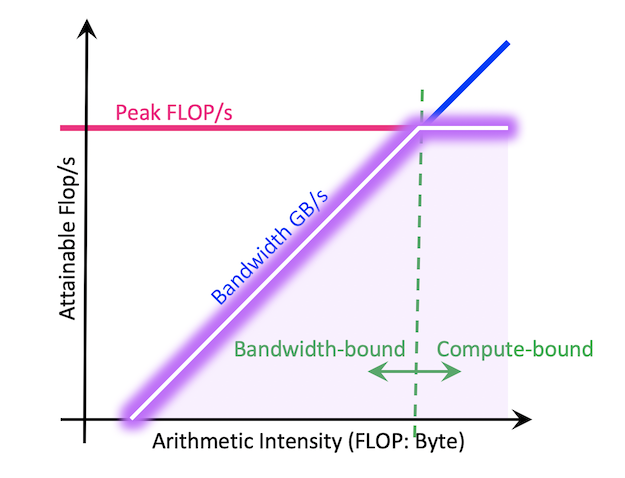
The Diagonal Line (Memory Wall): Represents the limit imposed by memory bandwidth (GB/s).
The Flat Ceiling (Compute Ceiling): Represents the peak TFLOPS of the device.
The Ridge Point (AI ≈ 10): The intersection where the diagonal meets the ceiling. This is the efficiency sweet spot, where the GPU is perfectly saturated — compute and memory access are perfectly balanced.

The Reality: Most local LLM decoding lives far to the left of this ridge, in the “memory-bound zone.” The bottleneck is the travel speed from HBM to the cores, leaving the majority of available compute idle.

3. Industry Standards: FlashAttention and PagedAttention

To break through this wall, modern engines use two primary architectural shifts:

FlashAttention: Tiling and Operator Fusion

Standard attention materializes a massive \(N \times N\) attention matrix in VRAM — an \(O(N^2)\) memory footprint — which is slow to read and write. FlashAttention (Dao et al., 2022) bypasses this via tiling and operator fusion:

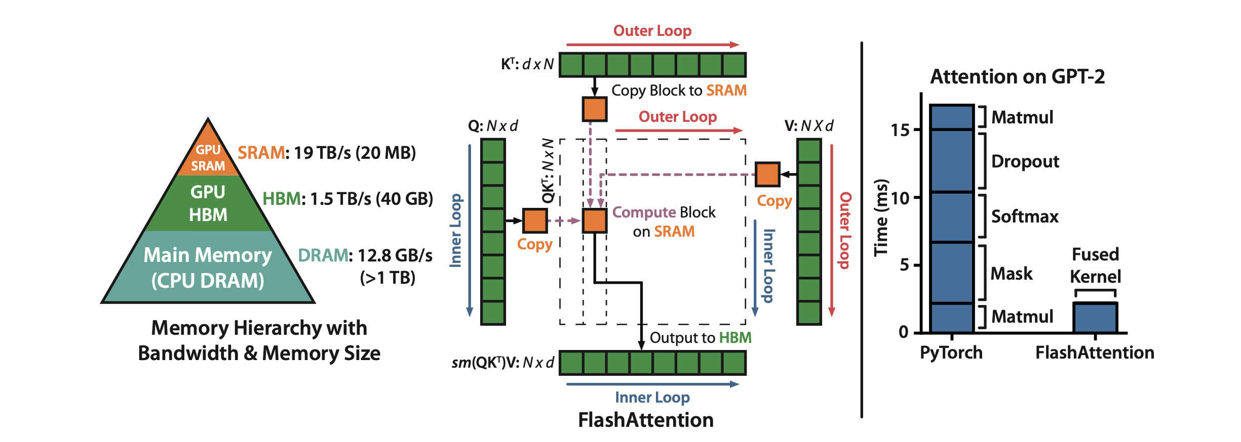
Tiling: The algorithm breaks the large \(Q, K, V\) matrices into smaller blocks (“tiles”) that fit entirely within the GPU’s SRAM — the fast on-chip buffer (~20MB on A100). Each tile computes a partial attention output independently.
Online Softmax & Accumulation: Instead of writing each tile’s intermediate result to HBM, FlashAttention uses an online softmax that incrementally combines tile outputs. At the end, all partial results are correctly summed to produce the exact full attention output.
Operator Fusion: The multiplication, softmax, and subsequent integration happen in a single kernel launch without writing intermediate results back to slow HBM.

PagedAttention: Memory Paging

Introduced by the vLLM team (Kwon et al., 2023), this technique solves the problem of KV cache fragmentation. Traditional systems pre-allocate a contiguous block of VRAM for each request large enough to hold the maximum possible sequence length.

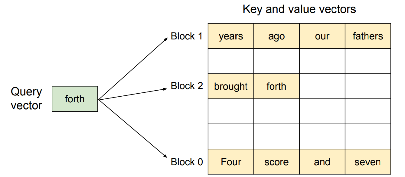
Internal fragmentation: If the actual sequence is shorter than the maximum, the over-allocated remainder is completely wasted — up to 50-60% of VRAM in practice.
External fragmentation: As requests complete and free their blocks, the VRAM heap becomes fragmented, making it hard to find contiguous space for new large requests.
PagedAttention solves this by borrowing the concept of virtual memory: a Block Table maps logical page numbers to non-contiguous physical VRAM blocks. Pages are allocated on demand (no over-allocation), and multiple sequences can share physical pages for common prefixes via Prefix Sharing.
Where it lives: PagedAttention sits in the attention mechanism’s KV cache management layer — it replaces the contiguous buffer with a page table lookup during the attention kernel.

4. Scaling the Reasoning Budget: MoE and CoT

Modern LLMs’ architectural traits demand even more resources, requiring tailored engines to accommodate their dynamic behavior efficiently:

Mixture of Experts (MoE)

Instead of a single monolithic Feed-Forward Network (FFN) per transformer layer, MoE models like Mixtral 8x7B use multiple “expert” FFN sub-networks and a Router (or gate) that selects which experts to activate for each token.

How it works, step by step: 1. Each token produces a hidden representation \(h\) before the FFN layer. 2. The Router computes a probability distribution over \(E\) experts: \(p = \text{softmax}(h \cdot W_r)\), where \(W_r \in \mathbb{R}^{d \times E}\). 3. Only the top-\(k\) experts (typically \(k=2\)) are activated for that token. 4. The token’s output is a weighted sum of the selected experts’ outputs: \(y = \sum_{i \in \text{top-k}} p_i \cdot \text{FFN}_i(h)\).

Chain of Thought (CoT) and the Thinking Parameter

Chain of Thought (Wei et al., 2022) prompts the model to produce intermediate reasoning steps before the final answer. This exponentially increases the number of decode tokens (\(m\)), making local generation speed the primary factor in whether an agent’s “thought process” takes 2 seconds or 20.

The “thinking” parameter shapes inference by modulating the stop condition: rather than stopping at the first answer token, the runtime allows the model to continue generating intermediate “thought” tokens until the budget is exhausted, then produces a final answer. This directly amplifies the memory-bound decode phase, making hardware efficiency even more critical.

Modern LLMs demand specific traits from inference engines

MoE and CoT/Thinking have transformed the inference surface from a uniform workload into a deeply heterogeneous one, and the gap is widening. Two consequences deserve to be made explicit before we get to Hermes-XLR:

MoE makes memory and compute disagree. A model like Mixtral 8x7B holds all 8 experts in VRAM (~\(96\) GB at FP16) but only computes \(\tfrac{k}{E} = \tfrac{1}{4}\) of them per token. The runtime has to schedule expert parallelism — place experts across devices — and minimize the all-to-all traffic that happens when the router’s top-\(k\) selection shifts mid-sequence. The memory and compute budgets live on different curves, and naive batching breaks both.
CoT/Thinking makes prefill and decode fight for the same GPU. A “small” request at prefill time can become a memory-bound decode problem for tens of seconds once thinking unlocks. Total wall-clock becomes \(\text{TTFT} + m \cdot \text{ITL}\) with \(m\) now routinely in the thousands. A runtime that treats prefill and decode as two serial phases will starve one of them.

On top of MoE and CoT, the modern inference stack layers even more moving parts, each one improving one metric (latency, throughput, memory) while making the kernel-selection problem \(n\)-dimensional:

Continuous batching (Orca, Yu et al., 2022) — fit new requests into slots vacated by finished ones, instead of waiting for the whole batch.
Weight quantization — INT4/INT8/FP8 with methods like AWQ (activation-aware) and SmoothQuant (migrate activation difficulty to weights).
KV-cache quantization — SqueezeBits, KV8 / KIVI, INT4 keys, FP8 values.
Speculative decoding alternatives — Medusa (parallel decoding heads) and EAGLE (feature-level draft) instead of a separate draft model.
Multi-LoRA serving — S-LoRA keeps thousands of adapters hot in VRAM with page-level swapping.
Heterogeneous offload — FlexGen pipelines GPU/CPU/NVMe tiers when the model does not fit.
Chunked prefill — interleave prompt tokens with decode steps to keep the GPU saturated instead of monopolizing it for hundreds of ms on long prompts.

Each of these is a powerful lever in isolation. The catch is that they are not orthogonal: enabling FP8 KV cache often forces you to abandon FlashAttention-2; turning on chunked prefill breaks certain continuous-batching implementations; quantizing a MoE’s router weights behaves differently from quantizing expert FFNs. The combinatorics explode.

That is exactly the problem the next section attacks. Hermes-XLR does not try to pick one technique — it picks a combination that fits the local hardware, the model, and the workload shape, and it does so automatically. This is the catharsis: one Capability Mapper, one Execution Plan, and the mess above disappears behind a stable, measurable interface.

5. Introducing Hermes-XLR: The Local Maximalist

Hermes-XLR is an optimization-first runtime built specifically for the hermes-agent framework and NVIDIA hardware. It uses a Capability Mapper to assess your hardware and emit a custom Execution Plan to saturate your specific VRAM and compute units.

Lever 1: Tiered Prefix Exploitation

Hermes Agent organizes prompts into three logical tiers: Stable (System), Context (History), and Volatile (Input). Because the Stable tier never changes, Hermes-XLR ensures a 100% cache hit rate, skipping the prefill phase entirely for every subsequent turn.

Lever 2: SMC-Speculative Decoding

Standard Speculative Decoding (SD) (Leviathan et al., 2022; Chen et al., 2023) uses a small “draft” model to propose \(\gamma\) tokens in a single forward pass, then the target model verifies all \(\gamma\) in parallel in one forward pass. The accepted prefix is committed; the first rejected token becomes the next decode position, and the rest of the draft is discarded. The expected accepted length is \(\frac{1 - \alpha^{\gamma+1}}{1 - \alpha}\) where \(\alpha\) is the per-token acceptance probability.

Why vanilla SD collapses on reasoning workloads. When draft and target distributions agree (\(\alpha \to 1\)), this is a near-perfect speedup: \(\gamma\) tokens at the cost of one target forward. But CoT and code generation create long-horizon regions where draft and target diverge: the draft confidently proposes a plausible-but-wrong token, the target rejects, and the entire \(\gamma\)-length draft is thrown away. You paid draft cost \(\gamma \times\) and recovered ~1 token. Empirically, \(\alpha\) can drop to ~0.3 on hard reasoning prompts, and the realized speedup falls below 1× — i.e. slower than no draft at all.

🧠 Particle-filter intuition: instead of betting on one sequence and rolling back, keep a population of \(N\) candidate continuations (“particles”). The draft model proposes one next token per particle (cost: \(N\) small forwards), the target scores all \(N\) in one batched forward, and we assign each particle a weight \(w^{(i)} = P_{\text{target}} / P_{\text{draft}}\). Low-weight particles are pruned; high-weight ones are replicated — survival of the fittest, exactly as in classical Monte Carlo filtering. The resampled population is an unbiased estimator of the target distribution, and because every particle already saw a target forward, the throughput is bounded from below even when \(\alpha\) is low.

Hermes-XLR implements Sequential Monte Carlo Speculative Decoding (SMC-SD) — a particle-filter approach that turns brittle single-shot speculation into a variance-controlled Monte Carlo estimator, which is a much better fit for the high-variance draft/target gap that reasoning models exhibit.

Initialization: Maintain \(N\) particles (candidate sequences), all starting at the current context.
Proposal: For each particle, the draft model proposes the next token \(x_{t+1}^{(i)}\).
Reweighting: Compute an importance weight for each particle: \[w^{(i)} = \frac{P_{\text{target}}(x_{t+1}^{(i)} \mid \text{context})}{P_{\text{draft}}(x_{t+1}^{(i)} \mid \text{context})}\] This weight measures how “surprised” the target model is by the draft’s proposal.
Resampling: Draw \(N\) new particles with replacement, where the probability of selecting particle \(i\) is proportional to \(w^{(i)}\). Particles with low weight (draft was wrong) are pruned; particles with high weight are replicated.
Result: The resampled particles form an unbiased approximation of the target model’s distribution. Effective throughput increases because idle compute is used to evaluate multiple candidate paths in parallel.

But particles are not free. Keeping \(N\) particles changes the effective batch size of the verification pass from \(1\) to \(N\). That moves the kernel rightward on the roofline toward higher arithmetic intensity — but at a hardware cost:

KV cache scales linearly with \(N\). Each particle carries its own context. For a 32K-token sequence on Llama-3-8B, the KV cache for a single sequence is already ~2 GB; with \(N{=}4\) particles, that grows to ~8 GB — on top of the model weights (~16 GB at FP16). On a consumer card like an RTX 4090 (24 GB VRAM), the budget disappears fast.
Activation memory rises with \(N\). The target batched forward pass must hold \(N\) copies of intermediate activations. Residual streams, attention scores, and hidden states all multiply by \(N\) during the verification step.
The draft/target FLOP ratio shifts. For small \(N\) (e.g. \(N{=}2\)), the draft cost dominates; for large \(N\) (e.g. \(N{=}16\)), the target verification pass dwarfs everything. There is a sweet spot where the marginal particle adds more accepted tokens than its KV and activation cost.

Hermes-XLR’s Capability Mapper handles this trade-off explicitly. Before enabling SMC-SD, it queries PagedAttention’s block table for the current context length and the free page count. \(N\) is set dynamically: when headroom is tight, \(N\) drops to 1 (degenerating to vanilla SD); when headroom is abundant, \(N\) climbs to exhaust the compute ceiling. The particle count becomes a dial that the Mapper turns based on remaining VRAM, not a hardcoded hyperparameter.

Lever 3: Latency Hiding

Recent updates introduce async persistence and safe read-only prefetch caching. These overlap non-inference tasks — like saving logs or updating agent history — with the GPU’s decode cycles, effectively “zeroing out” orchestration overhead from the critical path.

References

Papers

[1] Williams, S., Waterman, A., & Patterson, D. (2009). Roofline: An Insightful Visual Performance Model for Multicore Architectures. Communications of the ACM, 52(4). https://cacm.acm.org/research/roofline-an-insightful-visual-performance-model-for-multicore-architectures/

[2] Dao, T., Fu, D. Y., Ermon, S., Rudra, A., & Ré, C. (2022). FlashAttention: Fast and Memory-Efficient Exact Attention with IO-Awareness. NeurIPS 2022. https://arxiv.org/abs/2205.14135

[3] Kwon, W., Li, Z., Zhuang, S., Sheng, Y., Zheng, L., Yu, C. H., Gonzalez, J. E., Zhang, H., & Stoica, I. (2023). Efficient Memory Management for LLM Serving with PagedAttention. SOSP 2023. https://arxiv.org/abs/2309.06180

[4] Jiang, A. Q., et al. (2024). Mixtral of Experts. arXiv:2401.04088. https://arxiv.org/abs/2401.04088

[5] Shazeer, N., et al. (2017). Outrageously Large Neural Networks: The Sparsely-Gated Mixture-of-Experts Layer. arXiv:1701.06538. https://arxiv.org/abs/1701.06538

[6] Wei, J., et al. (2022). Chain-of-Thought Prompting Elicits Reasoning in Large Language Models. NeurIPS 2022. https://arxiv.org/abs/2201.11903

[7] Emara, Y., Seidel, K., Wang, H.-S., Wang, T.-H., Smolensky, P., Song, X., Pérez, E., & Kang, J. (2024). Faster LLM Inference via Sequential Monte Carlo. arXiv:2405.04437. https://arxiv.org/abs/2405.04437

[8] Leviathan, Y., Kalman, M., & Matias, Y. (2022). Fast Inference from Transformers via Speculative Decoding. arXiv:2211.17192. https://arxiv.org/abs/2211.17192

[9] Chen, C., et al. (2023). Accelerating Large Language Model Decoding with Speculative Sampling. arXiv:2302.01318. https://arxiv.org/abs/2302.01318

[10] Yu, G.-I., et al. (2022). Orca: A Distributed Serving System for Transformer-Based Generative Models. OSDI 2022. https://www.usenix.org/conference/osdi22/presentation/yu

[11] Lin, J., et al. (2023). AWQ: Activation-aware Weight Quantization for LLM Compression and Acceleration. arXiv:2306.00978. https://arxiv.org/abs/2306.00978

[12] Xiao, G., et al. (2022). SmoothQuant: Accurate and Efficient Post-Training Quantization for Large Language Models. arXiv:2211.10438. https://arxiv.org/abs/2211.10438

[13] Sheng, Y., et al. (2023). S-LoRA: Serving Thousands of Concurrent LoRA Adapters. arXiv:2312.13582. https://arxiv.org/abs/2312.13582

[14] Sheng, Y., et al. (2023). FlexGen: High-Throughput Generative Inference of Large Language Models with a Single GPU. ICML 2023. https://arxiv.org/abs/2303.06865

[15] Cai, T., et al. (2024). Medusa: Simple LLM Inference Acceleration Framework with Multiple Decoding Heads. arXiv:2401.10774. https://arxiv.org/abs/2401.10774

[16] Li, Y., et al. (2024). EAGLE: Speculative Sampling Requires Rethinking Feature Uncertainty. arXiv:2401.15077. https://arxiv.org/abs/2401.15077

[17] Guo, D., et al. (2025). DeepSeek-R1: Incentivizing Reasoning Capability in LLMs via Reinforcement Learning. arXiv:2501.12948. https://arxiv.org/abs/2501.12948

Figures

Figure 1. Prefill Phase (Compute-Bound) & Decode Phase (Memory-Bound) architecture diagrams. Inline SVG diagrams showing tensor flows for each phase.

Figure 2. Roofline Model — Attainable Performance vs. Arithmetic Intensity. Canonical roofline diagram showing memory wall (diagonal), compute ceiling (flat), and ridge point. Source: Williams et al. (2009), NERSC documentation. https://docs.nersc.gov/tools/performance/roofline/Roofline-intro.png

Figure 3. FlashAttention: Tiling & Operator Fusion of QK^T, Softmax, and PV. Schematic comparing standard attention (materializes N×N matrix in HBM) vs FlashAttention (streams Q/K/V tiles through SRAM, fuses softmax with matmul). Source: Dao et al. (2022), Tri Dao’s blog. https://tridao.me/blog/2022/09/flashattention.html

Figure 4. PagedAttention: Block Table Maps Logical KV Pages to Non-Contiguous VRAM. Original schematic showing logical KV buffer with block table redirecting to physical VRAM blocks, enabling prefix sharing. Source: Kwon et al. (2023), vLLM announcement. https://blog.vllm.ai/2023/06/20/vllm.html

Figure 5. Sparse Mixture-of-Experts — Router Activates Top-k of E FFNs per Token. Mixtral schematic: token hidden state scored by router against E expert FFNs; top-k computed and weighted-summed. Source: Jiang et al. (2024). https://arxiv.org/abs/2401.04088

Figure 6. The “Thinking” / Reasoning Budget Parameter in Modern CoT Models. Configurable thinking modes in QwQ-32B, DeepSeek-R1 implicit budget, and Chain-of-Thought origins. Sources: Qwen blog (2024), Guo et al. (2025), Wei et al. (2022).

Figure 7. SMC Speculative Decoding: Particle-Filter Loop (Proposal → Reweight → Resample). Emara et al.’s SMC-SD schematic: N particles proposed by draft, reweighted by w = P_target/P_draft, resampled for unbiased target approximation. Source: Emara et al. (2024). https://arxiv.org/abs/2405.04437

Additional Resources

Baseten. A Guide to LLM Inference and Performance. https://www.baseten.co/blog/llm-inference-guide
Nous Research. Architecture | Hermes Agent. https://github.com/NousResearch/hermes-agent
vLLM Team. Automatic Prefix Caching Documentation. https://docs.vllm.ai/en/latest/features/prefix_caching.html
NVIDIA Corporation. A100 and Hopper Architecture Datasheets. https://www.nvidia.com/en-us/data-center/a100/
SqueezeBits. vLLM vs TensorRT-LLM: KV Cache Quantization. https://squeezebits.com/blog/vllm-vs-tensorrt-llm-kv-cache-quantization
Nous Research. Hermes Skills System and /learn Command. https://github.com/NousResearch/hermes-agent/tree/main/skills
jeancmaia. hermes-xlr GitHub Repository. https://github.com/jeancmaia/hermes-xlr